The objective of creating drop-down list is to give an option to a user to select the option from the list.
so that it restricts the user to select unwanted entries input.
we can also use drop-down option for creating interactive dashboards for reporting purpose.
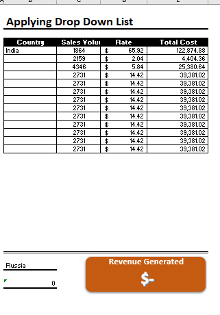
STEP 1 :- As we can see on the top we have a data entry form at the bottom we have a dashboard
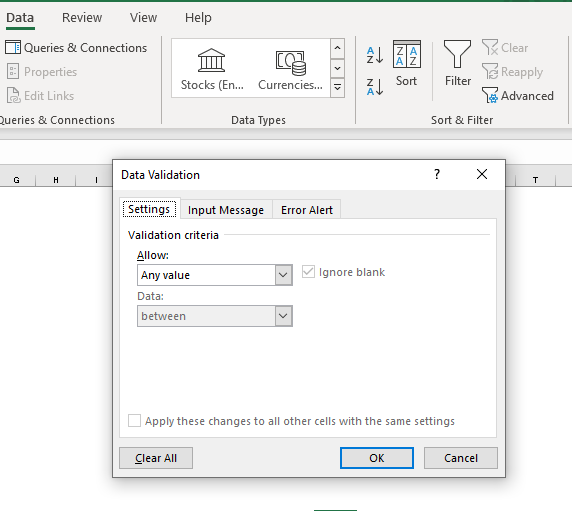
STEP 2 :- So for creating a drop-down list select a cell and go to data under this data there is data validation icon.
now click on the data validation and the screen will pop up shown below.
STEP 3 :- Now under the setting option click the allow button and select the list. now in source write the entries for eg india, united states, china etc we can add as many countries than click ok.
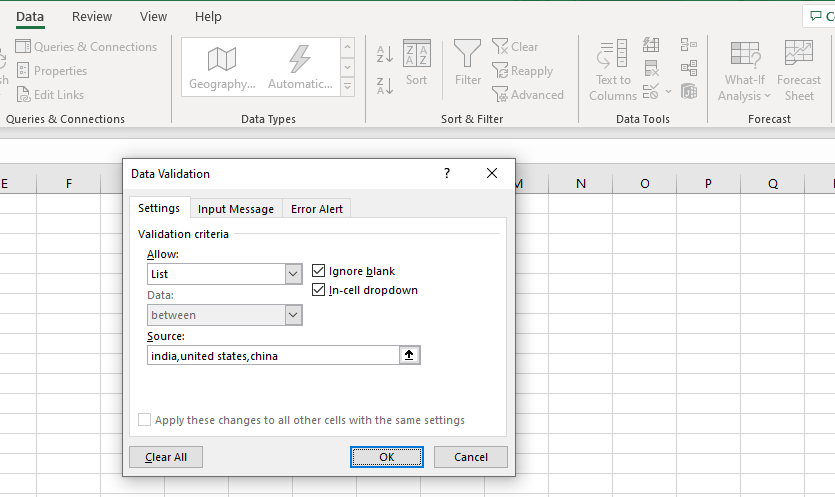
STEP 4 :- Now after this, if we select any cell there is a dropdown list of entries like India,united states, china, etc. so our drop-down list is updated.
Now let us understand how to create a drop-down from the list because whenever we have big data sets than it is not easy to write manually every entry. In this case, We will follow the steps given below.
Step 1: Select the cells containing the headings and values
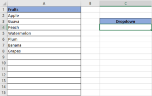
Step 2: Click on “Data” on the top of excel and select Data Validation:

Step 3: Select List under “Allow” and enter the Range of your data under “Source”. Click Ok:
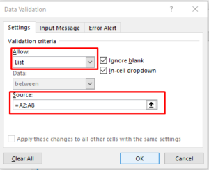
Note: In order to fix the range, you need to use “$” sign before Column and Row reference values i.e. $A$2:$A$8
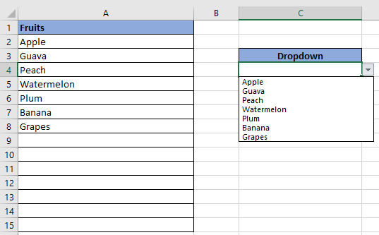
Step 4: Here is your drop down list:

Use Excel’s DATE function when you need to take three separate values and combine them to form a date.

This feature is particularly useful for summarizing data or improving the readability of complex sheets.

You need to know how to insert and use the degree symbol in a cell.
Let me explain why this is important. Yesterday, I was working with temperature data, and it was crucial to use the degree symbol to indicate Celsius and Fahrenheit.

Add new line in Excel cell lets you type on multiple lines within the same cell. Instead of having all the text in one long line, you can split it up to make it easier…
View two worksheets Side-by-Side in Excel lets you view multiple worksheets at once in layouts like vertical, horizontal, tiled, or cascade, so you don’t have to keep switching between sheets. You can also split a…

AVERAGE function is used to get the average of numbers. Function applies formula i.e. average = Sum of all values / (Divided by) number of items.