The AVERAGEIF function is used to get the “average” of values for a range of cells, based on multiple criteria.
The mathematical Average is calculated following: = Sum of all values / (divided by) number of items.
AVERAGEIF Function has two required arguments i.e. range, criteria and optional argument i.e. [average_range].
=AVERAGEIF(range,criteria,[average_range])
range argument is used to give the range of cells in which criteria needs to find
criteria argument is used to give criteria for average. We can give value (example “A”,”A*” >10, 50 ) or cell reference# (example: E2) in this argument
average_range argument is used to give cell range; those values to be averaged as per the criteria mentioned above
Kindly note, [average_range] is optional ONLY incase where range and [average_range] are in ONE column, but if, range and [average_range] are in DIFFERENT columns then [average_range] is NOT optional.
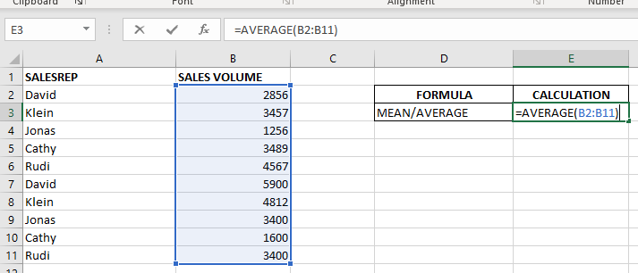
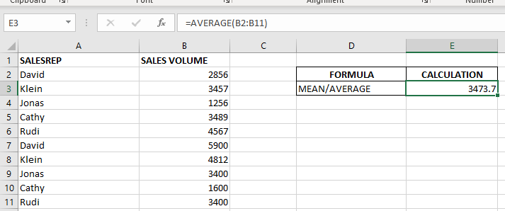
When we want to calculate the average with any condition than AVERAGEIF is used.
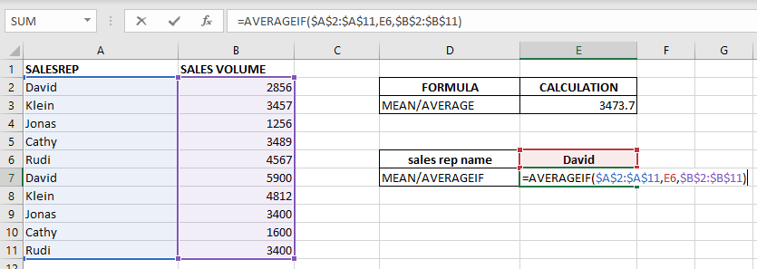
Here in example 2, we are calculating the average sales volume but with 1 condition, that’s why we will use AVERAGEIF here.
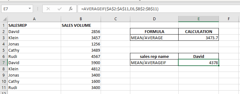
Formula:- =AVERAGEIF($A$2:$A$11,E6,$B$2:$B$11)
So here Criteria 1 is sales volume, the condition is David, and criteria 2 is a sales rep.
basically, we want to count the average of sales done by David.
The result is 4378 as shown in the 2nd image.
– Criteria argument can also work with Wild characters i.e. asterisk (*), question mark (?). Asterisk will find any series of characters and Question mark will find a single character.
– If you want to search actual * or ? (Asterisk or Question Mark) then type tilde (~) before * or ?
Hope you learnt this Function,
Don’t forget to leave your valuable comments!
If you liked this article and want to learn more similar tricks, please Subscribe us or follow us on Social Media by clicking below buttons:

In this tutorial, we’re going to explore one of the most intriguing features in Excel: the OFFSET function.
So, what is the OFFSET function in Excel? Simply put, OFFSET gives you a reference to a range of cells that’s moved from a starting point by a certain number of rows and columns.

Watch: How to use EOMONTH & EDATE Function in Excel? What is EOMONTH Function? The EOMONTH function in Excel returns the last day of a month based on a given date and a specified number of…

SUMIFS function is used to get the “total sum” of values for matching criteria across range. SUMIFS Function has required and optional arguments

How to Insert Symbol in Excel? I came across many queries regarding inserting special symbols in Excel. Here we are guiding how you may do this quickly in excel. Follow these steps and you may…
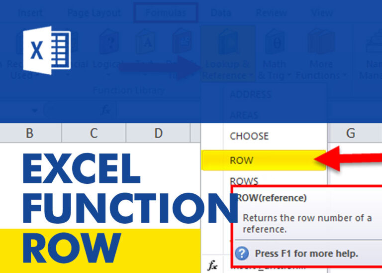
ROW function is used to get the row reference number of the excel worksheet. ROW Function has only one argument i.e. reference,

https://youtu.be/HmJL_y93pAs WEEKNUM function helps to calculate the week number of the given date in a year. It considers 1st January as first week by default and through the output for the given input date. Syntax:…