SEARCH function is used to find “position of character or text” in an available cell.
Search function is NOT case sensitive, means it will search “r” for text contains “r” and “R”. If you want to find value with case sensitive, then try FIND Function
=SEARCH(find_text,within_text,[start_num])
find_text argument, is the used to give character/ text or cell reference for which position is required to find
within_text argument, is used to give the cell reference from which find_value to be searched
[start_num] is optional argument and is used to specify the character from which search should be started. By default, the first character is 1, however if you want search should be started from 2nd find_text value then it should be position of 2nd find_text value and so on..
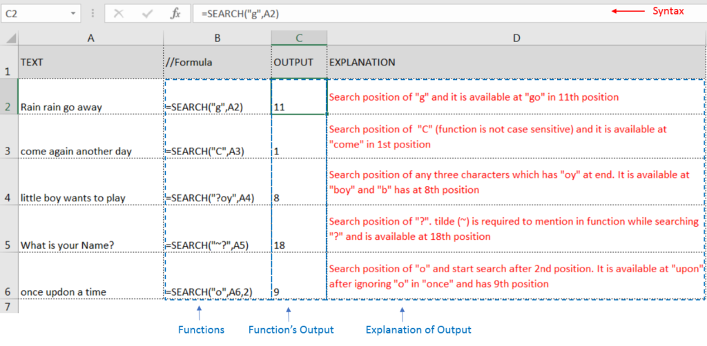
Here we have some examples, where:
– “Column A has various strings,
– “Column B” shows the sample formula that is applied,
– “Column C” shows the output of the function and
– Explanation is provided in Column “D”

– Search function will also work with Wild characters i.e. asterisk (*), question mark (?). Asterisk will find any series of characters and Question mark will find a single character.
– If you want to search actual * or ? (Asterisk or Question Mark) then type tilde (~) before * or ?
– Function should give output in “General” format, however if output is not as per the desired format then we need to change the cell format to “GENERAL”.
– If function parameters are not correctly applied in the function, then it will give output as “#VALUE!”
Don’t forget to leave your valuable comments!
If you liked this article and want to learn more similar tricks, please Subscribe us

AVERAGEIF function is used to get the “average” of values for matching criteria across range. Average = Sum of all values / number of items.

Watch Video: Rand and Randbetween Excel Functions Generate Random Numbers using Excel Functions We have got many instances where we needed to generate a random database or values. “RAND function” is very useful for users…

This tutorial explains how to use the IFERROR function in Excel to catch and handle errors. It shows you how to replace errors with a blank cell, a different value, or a custom message. You’ll also learn how to use IFERROR with functions like VLOOKUP and INDEX MATCH, and how it compares to other error-checking functions like IF ISERROR and IFNA

Watch: How to use VLOOKUP Function in Excel? What is VLOOKUP Function? The VLOOKUP function in Excel searches for a value in a table and returns a corresponding value from another column in the same row…

LARGE function is used to get the Largest k-th value from the range.
LARGE Function has two required arguments i.e. array, and k

COUNT function is used to get the total count of Number values in range or list.COUNT Function has one required and optional arguments.