SEARCH function is used to find “position of character or text” in an available cell.
Search function is NOT case sensitive, means it will search “r” for text contains “r” and “R”. If you want to find value with case sensitive, then try FIND Function
=SEARCH(find_text,within_text,[start_num])
find_text argument, is the used to give character/ text or cell reference for which position is required to find
within_text argument, is used to give the cell reference from which find_value to be searched
[start_num] is optional argument and is used to specify the character from which search should be started. By default, the first character is 1, however if you want search should be started from 2nd find_text value then it should be position of 2nd find_text value and so on..
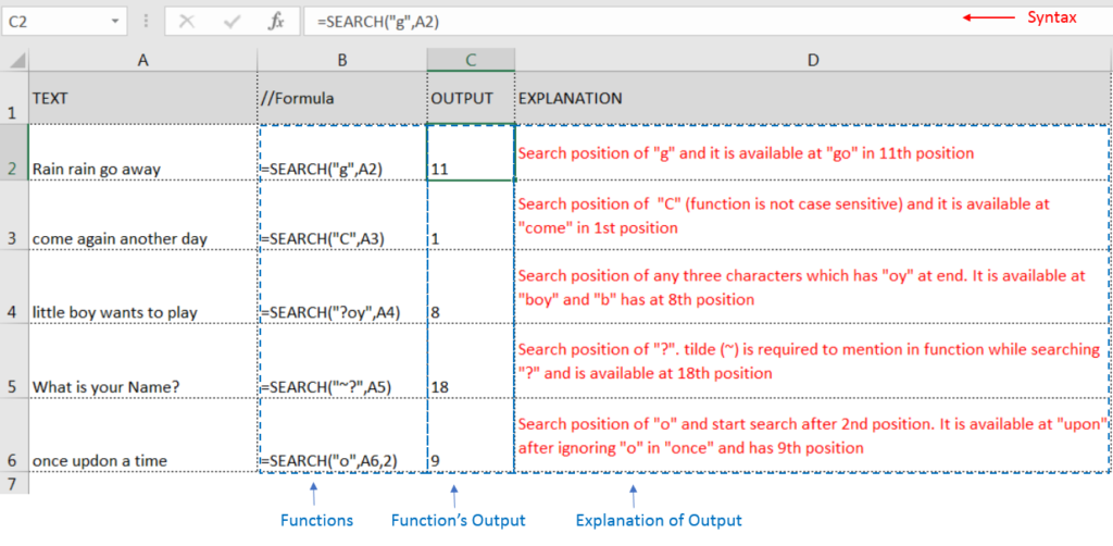
Here we have some examples, where:
– “Column A has various strings,
– “Column B” shows the sample formula that is applied,
– “Column C” shows the output of the function and
– Explanation is provided in Column “D”

– Search function will also work with Wild characters i.e. asterisk (*), question mark (?). Asterisk will find any series of characters and Question mark will find a single character.
– If you want to search actual * or ? (Asterisk or Question Mark) then type tilde (~) before * or ?
– Function should give output in “General” format, however if output is not as per the desired format then we need to change the cell format to “GENERAL”.
– If function parameters are not correctly applied in the function, then it will give output as “#VALUE!”
Don’t forget to leave your valuable comments!
If you liked this article and want to learn more similar tricks, please Subscribe us

https://youtu.be/HmJL_y93pAs WEEKNUM function helps to calculate the week number of the given date in a year. It considers 1st January as first week by default and through the output for the given input date. Syntax:…

The tutorial demonstrates how to find a date any number of days before or after today, counting either all days or only business days.

You must have faced a condition when your data cells contain extra spaces, leading spaces or trailing spaces and you wanted to remove these extra spaces to standardize the data. So here you may use…

AVERAGEIF function is used to get the “average” of values for matching criteria across range. Average = Sum of all values / number of items.

SUMIFS function is used to get the “total sum” of values for matching criteria across range. SUMIFS Function has required and optional arguments

In an “IF function” there will be two output i.e. TRUE or FALSE since either the statement will be “TRUE” or “FALSE”. If the statement is matching or correct, then output will be “TRUE” or if the statement is not matching or not correct then the output will be “FALSE