WEEKDAY as the word suggest it is “Day count in a week”. WEEKDAY function applies to a Date and returns the output for Day of the week. The output of the function varies from 0 to 7 and by default WEEKDAY function takes “Sunday to Saturday” as a week and counts Sunday as 1st Day till Saturday as 7th Day.
WEEKDAY Function has two arguments i.e. serial_number and return_type, are easy to apply and implement. Function should give output in number format, however if output is not as per the desired format then we need to change the cell format to “GENERAL”. We will be discussing the steps that how we can change the cell format to GENERAL in detail.
If input value is not in date format then the output of the function will return to “#VALUE!”. So always ensures that the input data range is in correct format to get the appropriate results/output.
WEEKDAY function is very advantageous in many ways. It helps for the document where weekday sequencing is required in more often. Applying weekday count manually (one by one) to a report is very difficult and WEEKDAY Function helps to apply the function in large database at once and makes the work easy, saves time and increases efficiency.
WEEKDAY Function is very useful and can be used in many places. Like it can be used as follows:
– Preparing employees and wages summary, where wages are paid weekly
– Employees utilization or productivity, attendance tracker on weekly basis
– Or any other database where there is requirement of count of days in a week, WEEKDAY Function” can be used
=WEEKDAY(serial_number,[return_type] )
There are two arguments i.e. serial_number and return_type. Below are the details of each arguments:
serial_number argument, is used to give cell reference where date is mentioned and weekday to be counted.
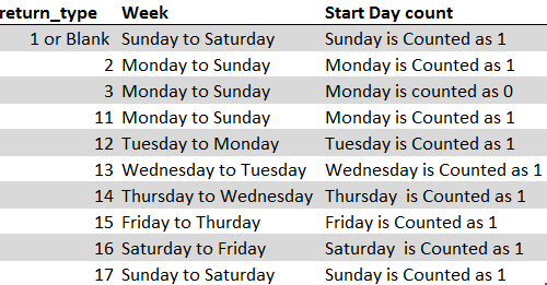
return_type [Optional] argument, is a optional argument is used to give reference to selection of week period. by default it takes “Sunday to Saturday” as a week and counts Sunday as 1st Day till Saturday as 7th Day, however if week period is different than “Sunday to Saturday” return type argument can be used.
Below is the list of return_type and explanation:

Suppose we have a date i.e. Monday, 23rd March 2020 and need to identify what is count of week for the said date. We will be using the default week i.e. Sunday to Saturday while applying the function.

Explanation: We can see the output of the function returns as 2. Because while considering a week of Sunday to Saturday, Sunday is 1st day and Monday is 2nd Day.
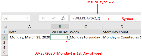
With the same date i.e. Monday, 23rd March 2020 and need to identify what is count of week for the said date. We will be considering “return type = 2” i.e. Monday to Sunday while applying the function.

Explanation: We can see the output of the function returns as 1. Because while considering a week of Monday to Sunday, Monday is 1st day.
Here we are evaluating a date i.e. Monday, 23rd March 2020 with All “return type” argument

Explanation: We can see the output of the function with various “return_type” returns value between 0 to 7.
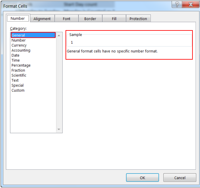
If output is not as per the desired format then we need to change the cell format to “GENERAL”. Follow below steps to change the format of the cell:
Step 1: Select the Cell or Data Range
Step 2: Press Ctrl + 1 to open “Format Cells” option
Step 3: Select the option to “General”

This will change the format of the cell to desired format.
Hope you learnt this Function!
Don’t forget to leave your valuable comments!
If you are liking our articles and want to learn more similar tricks, please Subscribe us

COUNTA function is used to get the total count of Any-value or Non-Blanks in range. COUNTA Function has one required and optional argument: value1, value2

MATCH function performs lookup for a value in a range and returns its position sequence number as output. It has two required and one optional arguments

Microsoft Excel “TODAY” function is used to get the current Date. It is very useful function and can be used in many ways. “TODAY Function” does not have any argument that makes this easy to apply and implement.

In an “IF function” there will be two output i.e. TRUE or FALSE since either the statement will be “TRUE” or “FALSE”. If the statement is matching or correct, then output will be “TRUE” or if the statement is not matching or not correct then the output will be “FALSE

This tutorial explains how the TRANSPOSE function works and shows you the right way to use it to switch data in Excel.
Everyone has different preferences, even for work habits. Some people like to arrange data in vertical columns, while others prefer horizontal rows. If you ever need to switch the direction of your data quickly, the TRANSPOSE function can help

This guide shows how to use the nested IF function in Excel to check several conditions. You will also learn about other functions that can be to use than a nested formula.
When you want to make decisions in Excel, you often use an IF formula. It checks if something is true, then gives one result if it is and another result if it isn’t. If you need to check more than one thing, you can put many IFs inside each other.
Although using multiple IFs is common, it’s not the only way to check several conditions in Excel. This guide will introduce you to some easier and useful alternatives.