Comparing Columns in Microsoft excel is much often feature that is used while managing database. We have many ways to compare the columns in excel and can be used as per the requirement. We will be learning them in very easy and simple steps in below section..
Here we have two data sets and need to match the names available in column A with column B and identify the values which are matching or not matching with each other. We will be using a syntax to get the desired output.
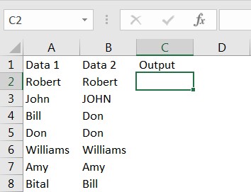
Syntax: =Cell1=Cell2
Here Cell1 and Cell2 are the data cell range that we are comparing with each other. This is very simple and gives results in “TRUE” and “FALSE” format. “TRUE” means that value is matching with each other, whereas “FALSE” says value is not matching.
Things To Remember
We need to remember that above function is not “Case Sensitive”, means “John” and “JOHN” will be considered as cells are matching with each other and output of function will be “TRUE”
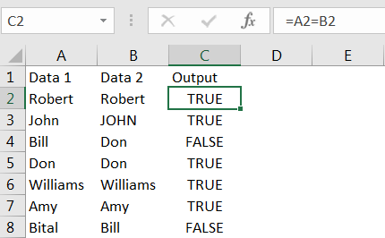
Column C represents the output, where values in Column A and B are compared. We can see the output, in cell C2 shows “True” i.e. “Robert” is matching in cell A2 and B2.
Also, name “John” (cell A3) and “JOHN” (cell B3) are considered as matched and output is “TRUE”. Values in cell A4 (Bill) and B4 (Don) are not matching that is why output is “FALSE”
Syntax: =(Cell1=Cell2) is not Case Sensitive means “John and JOHN” will be considered as “TRUE”. However, if we need to compare the database to exact match means, name “John” and “JOHN” should be considered as two then we need to follow equal function along with “Exact”
Syntax: =Exact(A2,B2)
Here “Exact” excel function is used to compare the exact values, “A2, B2” are the cells comparing with each other. Output of the syntax will be “TRUE or FALSE”. “TRUE” means that value is matching whereas “FALSE” says that value is not matching.
Things To Remember
We need to remember that above function is “Case Sensitive”, means “John” and “JOHN” will be considered as “FALSE”
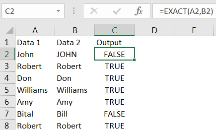
Column C represents the output, where values in Column A and B are compared. We can see the output, in cell C2 shows “FALSE” because “John (cell A2)” and “JOHN (cell B2)” are considered as not matching
Sometimes we need to customize the output, means instead of “TRUE” or “FALSE” if we need any other output to be shown then we need to use the equal function along with “IF”.
For example, if we need “Name is Matching” text instead of “TRUE” and “Name is not Matching” text instead of “FALSE” then we need to follow below:
Syntax: =IF(A2=B2,"Name is Matching", "Name is not Matching")
Here “IF” excel function is used to get the customized result. We are comparing cells “A2, B2” and if both cells are matching then output will be “Name is Matching” whereas if cells are not matching then output will be “Name is not Matching”
Things To Remember
We need to remember that we can customize the output to any text, means instead of “Name is Matching, or Name is not Matching” we can mention like “Result is Matching, or Result is not Matching”
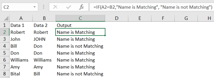
Column C represents the output, where values in Column A and B are compared. We can see the output, in cell C2 shows “Name is Matching” because “Robert (cell A2)” and “Robert (cell B2)” are matching.
We can also highlight the duplicate values in the database using Conditional Formatting. This is very effective option to bring the duplicate values out within few steps. We can choose any color and formatting to highlight the values of the database. Follow the below steps to explore:
> Select the Data Range:
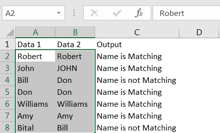
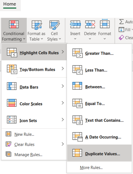
> Click to Hone Menu -> Conditional Formatting -> Highlight Cells Rules -> Duplicate Values..
> Select to “Duplicate” and values with, choose the appropriate formatting of your choice. Default option is selected, i.e. “Light Red Fill with Dark Red Text”
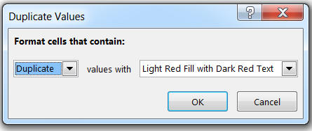
> Click to “OK”
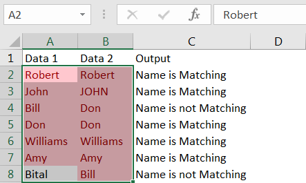
Report will be highlighted as above. Results can be seen that all the duplicate values in the Selected Data Range is highlighted to the Formatting provided.
We can also highlight the unique values in the database using Conditional Formatting.
Follow the similar steps as “Duplicate” values, just select “Unique” in the below option provided
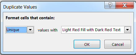
Click to “OK”
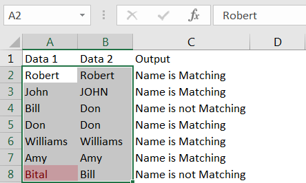
Report will be highlighted as above. Results can be seen that all the Unique values in the Selected Data Range is highlighted to the Formatting provided.

This article has Top Excel Interview Questions and Answers to test your Excel skills. It’s great for beginners who are just starting out, or even pros who want a refresher. The questions cover everything you might need for jobs like data analyst, business analyst, or accountant.
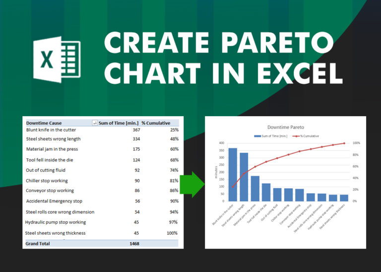
What is Pareto Chart? Pareto principle was introduced by Italian Economist Vilfredo Pareto. He stated that 80% of the effects are caused by 20% of the causes. So if we closely monitor and solve 20% of…

This video will help you to understand how you may use conditional formatting to highlight row based on conditions. Subscribe us for more updates

You need to know how to insert and use the degree symbol in a cell.
Let me explain why this is important. Yesterday, I was working with temperature data, and it was crucial to use the degree symbol to indicate Celsius and Fahrenheit.

Undo in excel very useful If you’re new to Excel or even if you’ve been using it for a while, you’ve probably made a mistake on a spreadsheet. Mistakes happen a lot, especially when working…

Group worksheets in Excel makes it easier to manage a big workbook. This feature allows you to treat multiple worksheets as one, helping you perform identical tasks like formatting or data entry across several sheets…