When I started my career in working with excel dashboards, I always used to face most common challenge in “Data Validation” technique where I want a smart data validation to avoid all blank cells and keep adding and deleting the values from drop down dynamically.
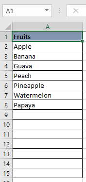
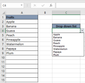
Step 1: Identify the range which you want to show into data validation list. Here I selected a range from A2:A15. Refer the below screenshot:
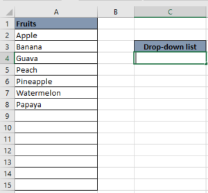
Step 2: I will be creating a dynamic drop down list using above Range (A2:15) and applying this validation to Cell “C4” as below:

Step 3: Here we will be using “OFFSET” function to create dynamic drop down list:
“=OFFSET(reference, rows, cols, [height], [width])”
Note: Click here “OFFSET” to learn this function in detail
Parameters:
Reference: This is a range which we will be using and adjusting. So here it is “$A$2:$A$15”
Rows: As our base row starts from “2” and our data also starts from $A$2. Therefore, we should not be using this parameter
Cols: As we will be adjusting the same column and no need to shift data anywhere on the sheet Therefore, we should not be using this parameter
Height: We are going to adjust the height of our data in current example which starts from $A$2 and ends at $A$15. So it depends on the data filled. Currently we have data till 8th Row. We will calculate the height until filled cell by using COUNTA function
Note: Click here “COUNTA” to learn this function in detail
Width: We do not have width of the data, so can leave this as well
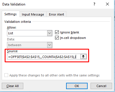
So below is our final formula: “=OFFSET($A$2:$A$15,,,COUNTA($A$2:$A$15),)”
Step 4: Select “C4” cell and create “Data Validation” list by pasting the formula under “Source” as below:
Click “OK”
Note: You can create a named range by using the same formula and then may use that named range instead of pasting the formula under data validation list
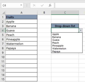
Step 5: Here is your Validation list
Note: Click here “Data Validation” to learn this feature in detail
And once you add a new value in “A9” cell, it will automatically added to drop down list as below:
Hope you enjoyed this article. See you soon again with a new article 
Introduction Welcome to this comprehensive guide on using Power Query in Excel to split data efficiently. In this tutorial, we’ll walk you through the step-by-step process of splitting columns, specifically focusing on splitting the name…

Microsoft Excel lets you share your spreadsheets with others, but sometimes your co-workers might edit the wrong column by mistake. To avoid this, you can lock specific columns. In this guide, we’ll show you how…

Conditional Formatting helps to easily identify the usual and unusual numbers/ conditions, creating interactive visualization by means of Highlight Cells by Rules, Top/Bottom Rules, Data Bars, Color Scales and Icon Sets.
Have you ever got into situation in office where you need to count the cells in Excel sheet with specific color? If yes then you can use following code which counts the number of cells…

Few Excel Tips 1. CHANGE DIRECTION WHEN YOU PRESS ENTER Whenever you press enter, you must be thinking why my cell selection shifts down. Why it can’t go UP, Down, Left. Surprised This is very…

Microsoft Excel helps you organize and work with data in many ways. When you have a lot of information or need to break it into parts, splitting cells is very useful. Splitting cells means taking the content of one cell and dividing it into multiple cells. This can be especially helpful for separating names, addresses, or other data that are combined in one cell. Learn how to split cells in Excel using its built-in functions and formulas.