The objective of creating drop-down list is to give an option to a user to select the option from the list.
so that it restricts the user to select unwanted entries input.
we can also use drop-down option for creating interactive dashboards for reporting purpose.
STEP 1 :- As we can see on the top we have a data entry form at the bottom we have a dashboard
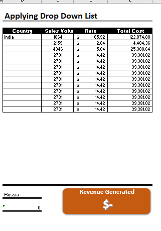
STEP 2 :- So for creating a drop-down list select a cell and go to data under this data there is data validation icon.
now click on the data validation and the screen will pop up shown below.
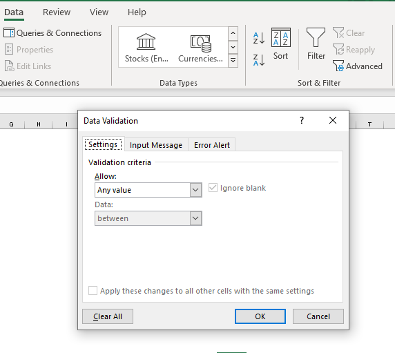
STEP 3 :- Now under the setting option click the allow button and select the list. now in source write the entries for eg india, united states, china etc we can add as many countries than click ok.
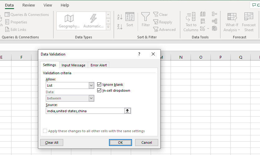
STEP 4 :- Now after this, if we select any cell there is a dropdown list of entries like India,united states, china, etc. so our drop-down list is updated.
Now let us understand how to create a drop-down from the list because whenever we have big data sets than it is not easy to write manually every entry. In this case, We will follow the steps given below.
Step 1: Select the cells containing the headings and values
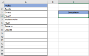
Step 2: Click on “Data” on the top of excel and select Data Validation:

Step 3: Select List under “Allow” and enter the Range of your data under “Source”. Click Ok:
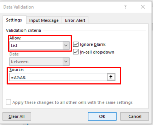
Note: In order to fix the range, you need to use “$” sign before Column and Row reference values i.e. $A$2:$A$8
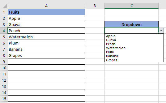
Step 4: Here is your drop down list:

You need to know how to insert and use the degree symbol in a cell.
Let me explain why this is important. Yesterday, I was working with temperature data, and it was crucial to use the degree symbol to indicate Celsius and Fahrenheit.

Learn how to insert and use checkboxes in Excel. Find out how to change text value, link check boxes to cell and formatting of check boxes.

LOWER function is used for changing the format of any text or string to LOWER case.

AVERAGEIF function is used to get the “average” of values for matching criteria across range. Average = Sum of all values / number of items.

This tutorial shows you three easy ways to add hyperlinks in Excel. You will learn how to insert, change, and remove hyperlinks in your worksheets. It also explains how to fix links that don’t work.
Hyperlinks are often used on the internet to move between websites. In Excel, you can create links like that too. You can make a link to another cell, a different sheet, or even another workbook. You can also link to open a new Excel file or start an email message. This guide will show you how to do all of this in Excel 2016, 2013, 2010, and older versions.

This tutorial explains a new Excel 365 function that helps you make an array bigger to the size you want by filling it with a chosen value. Do you need to expand an array to…