The objective of creating drop-down list is to give an option to a user to select the option from the list.
so that it restricts the user to select unwanted entries input.
we can also use drop-down option for creating interactive dashboards for reporting purpose.
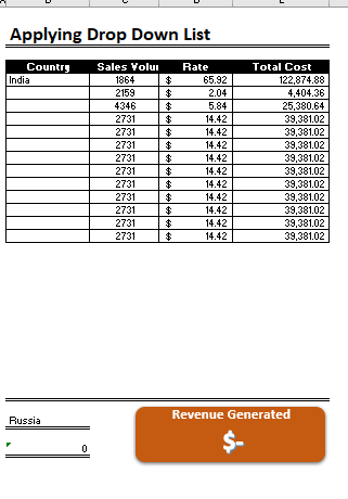
STEP 1 :- As we can see on the top we have a data entry form at the bottom we have a dashboard
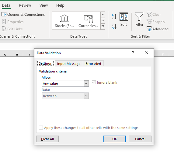
STEP 2 :- So for creating a drop-down list select a cell and go to data under this data there is data validation icon.
now click on the data validation and the screen will pop up shown below.
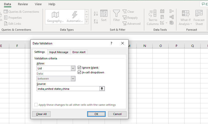
STEP 3 :- Now under the setting option click the allow button and select the list. now in source write the entries for eg india, united states, china etc we can add as many countries than click ok.
STEP 4 :- Now after this, if we select any cell there is a dropdown list of entries like India,united states, china, etc. so our drop-down list is updated.
Now let us understand how to create a drop-down from the list because whenever we have big data sets than it is not easy to write manually every entry. In this case, We will follow the steps given below.
Step 1: Select the cells containing the headings and values
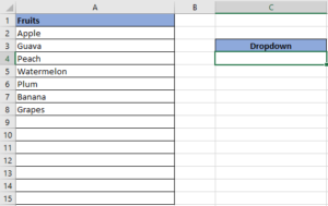
Step 2: Click on “Data” on the top of excel and select Data Validation:

Step 3: Select List under “Allow” and enter the Range of your data under “Source”. Click Ok:
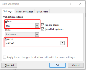
Note: In order to fix the range, you need to use “$” sign before Column and Row reference values i.e. $A$2:$A$8
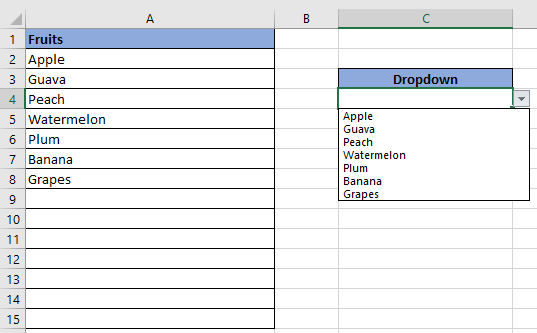
Step 4: Here is your drop down list:

Excel Dark mode reduces eye strain and makes the screen more comfortable to work on in high-contrast settings. Follow this easy tutorial to enable dark mode for both the Excel interface and the spreadsheet cells.

What is Excel Tables? Excel tables organize data into rows and columns with special features like unique names for columns, easy-to-use formulas, automatic formatting, and simple sorting and filtering. They make data management and analysis…

This step-by-step tutorial empowers you to leverage Power Query’s robust filtering capabilities. Learn to filter by date, text, numbers, and more, streamlining your workflow and unlocking deeper insights from your data. Watch now and elevate your Excel expertise!
Use Excel’s DATE function when you need to take three separate values and combine them to form a date.

FIND function is used to find the position of text, or character in an available string.
If you want to print your Excel spreadsheets with gridlines, this guide is for you. Adding gridlines makes your data easier to read and gives your spreadsheet a clean, organized look. In this post, we’ll…