The objective of creating drop-down list is to give an option to a user to select the option from the list.
so that it restricts the user to select unwanted entries input.
we can also use drop-down option for creating interactive dashboards for reporting purpose.
STEP 1 :- As we can see on the top we have a data entry form at the bottom we have a dashboard
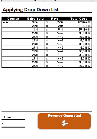
STEP 2 :- So for creating a drop-down list select a cell and go to data under this data there is data validation icon.
now click on the data validation and the screen will pop up shown below.
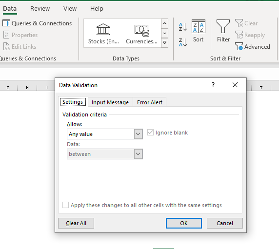
STEP 3 :- Now under the setting option click the allow button and select the list. now in source write the entries for eg india, united states, china etc we can add as many countries than click ok.
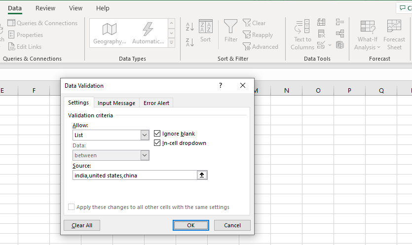
STEP 4 :- Now after this, if we select any cell there is a dropdown list of entries like India,united states, china, etc. so our drop-down list is updated.
Now let us understand how to create a drop-down from the list because whenever we have big data sets than it is not easy to write manually every entry. In this case, We will follow the steps given below.
Step 1: Select the cells containing the headings and values
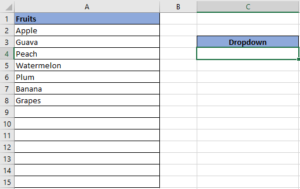
Step 2: Click on “Data” on the top of excel and select Data Validation:

Step 3: Select List under “Allow” and enter the Range of your data under “Source”. Click Ok:
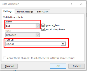
Note: In order to fix the range, you need to use “$” sign before Column and Row reference values i.e. $A$2:$A$8
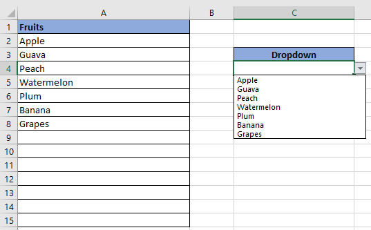
Step 4: Here is your drop down list:

If you have data on paper that you want to add to Excel, you can take a photo of it, save the photo to your computer, and upload the data into Excel. This saves time…

XLOOKUP can find a value that matches exactly or is the closest approximation. It can also look to the left, right, or both, which is an alternative to the VLOOKUP function
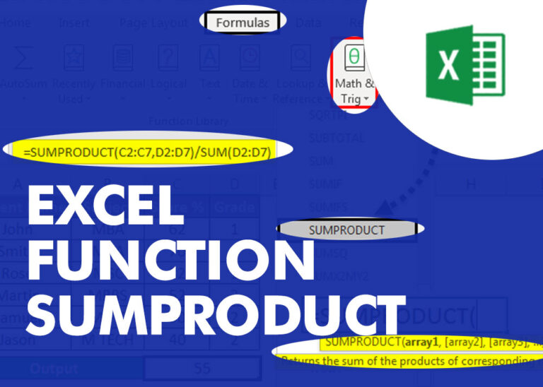
SUMPRODUCT function performs multiplication of numbers within arrays and then sum the values SUMPRODUCT function has array1, 2.. arguments.

While starting Excelsirji.Com, it is always been critical for me to find the best to amaze the viewer experience. So I spent many hours on web to read, explore amazing excel content which I really…

LEFT function is used for extracting the “Left Most” characters from the available string. The output of the function returns the extracted characters in new cell

This video will help you to understand how you may use conditional formatting to highlight row based on conditions. Subscribe us for more updates