As Microsoft is releasing new versions of Excel after every few years, they are working on adding more and more features in the application to support increased user demands. There are hundreds of formulas/functions available in Excel which can be used to get any type of information from the data.
Have you ever felt that Microsoft should have added a formula in Excel which can count the cells based on specific color? I have seen many code requests to share a VBA code that can count the cells by its color.
To help our subscribers and developers, we are sharing 2 codes that be used to count the cells with specific color and returns the count of the matching color cells.
					Public Function CountByColor(rng As Range, Red As Long, Green As Long, Blue As Long) As Long

    'Variable declaration
    Dim lCount As Long
    Dim rngCell As Range

    'Loop throught each cell in the range
    For Each rngCell In rng
        'Checking and count color
        If rngCell.Interior.Color = RGB(Red, Green, Blue) Then
            lCount = lCount + 1
        End If
    Next

    'Return the value
    CountByColor = lCount

End Function
					Public Function CountByColor(rng As Range, ColorCell As Range) As Double

    'Variable declaration
    Dim lCount As Long
    Dim rngCell As Range

    'Loop throught each cell in the range
    For Each rngCell In rng
        'Checking and count color
        If rngCell.Interior.Color = ColorCell.Interior.Color Then
            lCount = lCount + 1
        End If
    Next

    'Return the value
    CountByColor = lCount

End Function
If you want to use this code in your VBA tool, then follow below steps:
Step 1: Open the Excel file in which you want to copy this code
Step 2: Press Alt+F11 to open VBA editor
Step 3: Insert a new module from Insert > Module menu
Step 4: Paste the code in the module
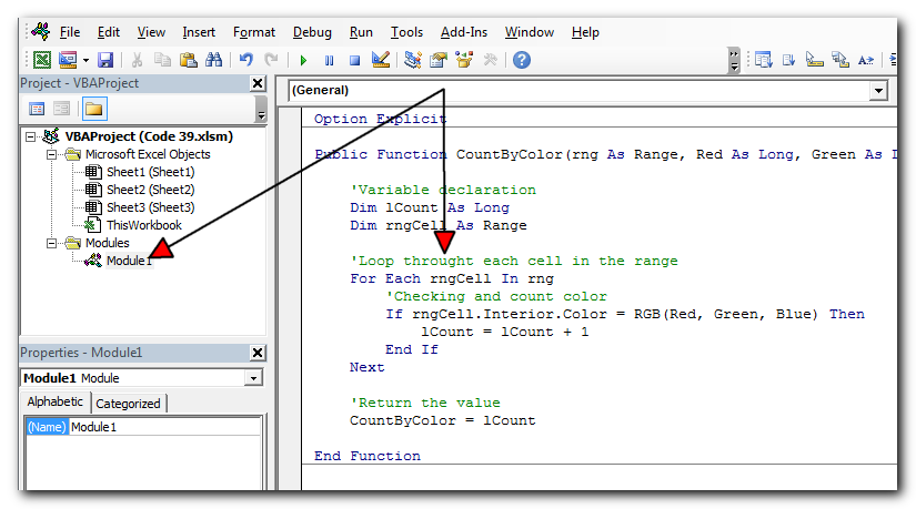
Step 5: Now you are ready to use this code as Excel Function/Formula
Step 6: Type the formula in the cell where you want to get the count of specific colored cells
First Code Example:=CountByColor(A2:A11,146, 208, 80)
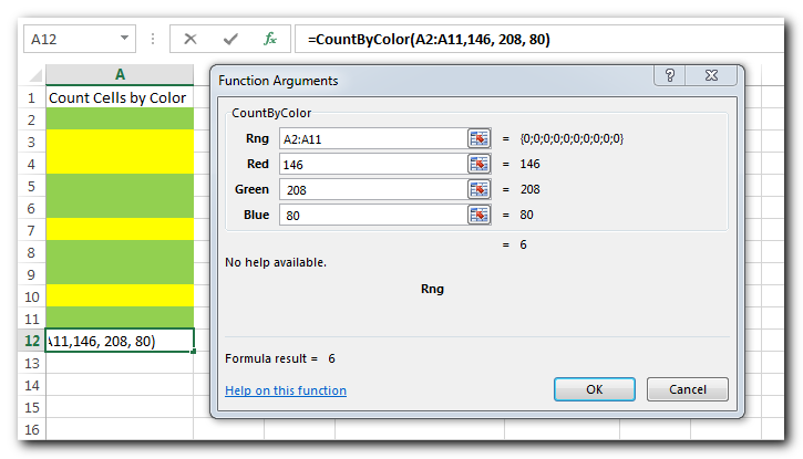
The first parameter of the formula is the range from which you want to count the specific color cells. The second, third and fourth parameters are RGB code of the color.
Second Code Example:=CountByColor(A2:A11,A8)
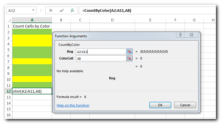
The first parameter of the formula is the range from which you want to count the specific color cells. The second parameter is the cell from which you want to compare the color.
In the first VBA code, we have used RGB color codes to find the matching cells and sum the values. You can find RGB codes of any color using following steps:
Step 1: Select the cell which contain the color you want to use
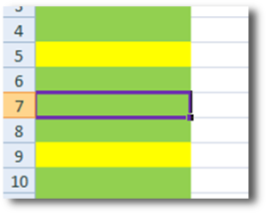
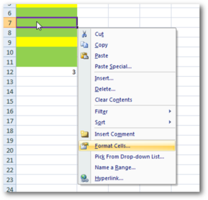
Step 2: Right click and select ‘Format Cells…’
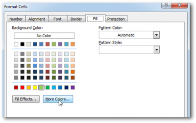
Step 3: In the Format Cells dialog box go to ‘Fill’ tab and click on ‘More Colors…’
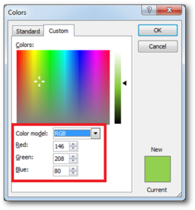
Step 4: That’s all, in the ‘Color’ dialog box, you can view the RGB (Red, Green, Blue) codes of the color
Thanks for reading the article, subscribe us to get more VBA tricks

This Excel VBA Code converts the excel range into HTML and also can convert Excel to HTML Table to paste data on Outlook Email Body

This guide explains the basics of Excel’s Advanced Filter and shows you how to use it to find records that match one or more complicated conditions.
If you’ve read our previous guide, you know that Excel’s regular filter offers different options for filtering text, numbers, and dates. These options work well for many situations, but not all. When the regular filter isn’t enough, you can use the Advanced Filter to set up custom criteria that fit your exact needs.
Excel’s Advanced Filter is especially useful for finding data based on two or more complex conditions. For example, you can use it to find matches and differences between two columns, filter rows that match another list, or find exact matches with the same uppercase and lowercase letters.
Advanced Filter is available in all Excel versions from 365 to 2003. Click the links below to learn more.
This tutorial shows you how to change the row colors in Excel to automatically highlight every other row or every nth row or column in your worksheets. You will also learn how to use Excel’s banded rows and columns and find some helpful formulas to shade rows based on value changes.
Using alternating colors for rows in Excel is a common way to make data easier to read. While it’s simple to manually highlight rows in a small table, it can be very time-consuming in larger tables. A better approach is to automatically alternate the colors of rows or columns, and this article will show you how to do it quickly

Outlook Email Management Tool is an Excel based tool which works with Outlook 2010 or above version and helps you to read, copy or move multiple emails from an Outlook folder and sub-folders on click of a button. The tool also supports extracting attachments from emails as well.

Learn to reduce excel file size. Tips include removing unnecessary formatting, compressing images, using formulas instead of hardcoded data, and optimizing pivot tables. Clearing unused cells and minimizing data ranges also help. Lastly, consider saving as binary or using third-party add-ins for further compression.

Table of Content How does testing help? How should I test my tool or application? How does Dummy Data Generator tool helps in testing? How do I use this tool? From many years I have…
This helped heaps thank you very much! I now I am wondering how do I write up a VBA code to auto-update or simultaneously count cells by color when I am doing color coding my cells. Cheers
Place the code in Worksheet change event (the sheet) where you want to use this.