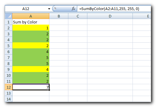
Recently some of our subscribers have requested us to share a VBA code that can sum the cells by its color. To help our subscribers and developers, we are sharing 2 codes that be used to sum the cells with specific color and returns the total sum of the matching color cells
Public Function SumByColor(rng As Range, Red As Long, Green As Long, Blue As Long) As Double

    'Variable declaration
    Dim dblSum As Double
    Dim rngCell As Range

    'Loop throught each cell in the range
    For Each rngCell In rng
        'Checking and sum color
        If rngCell.Interior.Color = RGB(Red, Green, Blue) Then
            If IsNumeric(rngCell.Value) = True Then
                dblSum = dblSum + rngCell.Value
            End If
        End If
    Next

    'Return the value
    SumByColor = dblSum

End FunctionPublic Function SumByColor(rng As Range, ColorCell As Range) As Double
'Variable declaration
Dim dblSum As Double
Dim rngCell As Range
'Loop throught each cell in the range
For Each rngCell In rng
'Checking and sum color
If rngCell.Interior.Color = ColorCell.Interior.Color Then
If IsNumeric(rngCell.Value) = True Then
dblSum = dblSum + rngCell.Value
End If
End If
Next
'Return the value
SumByColor = dblSum
End Function
Step 1: Open the Excel file in which you want to copy this code
Step 2: Press Alt+F11 to open VBA editor
Step 3: Insert a new module from Insert > Module menu
Step 4: Paste the code in the module
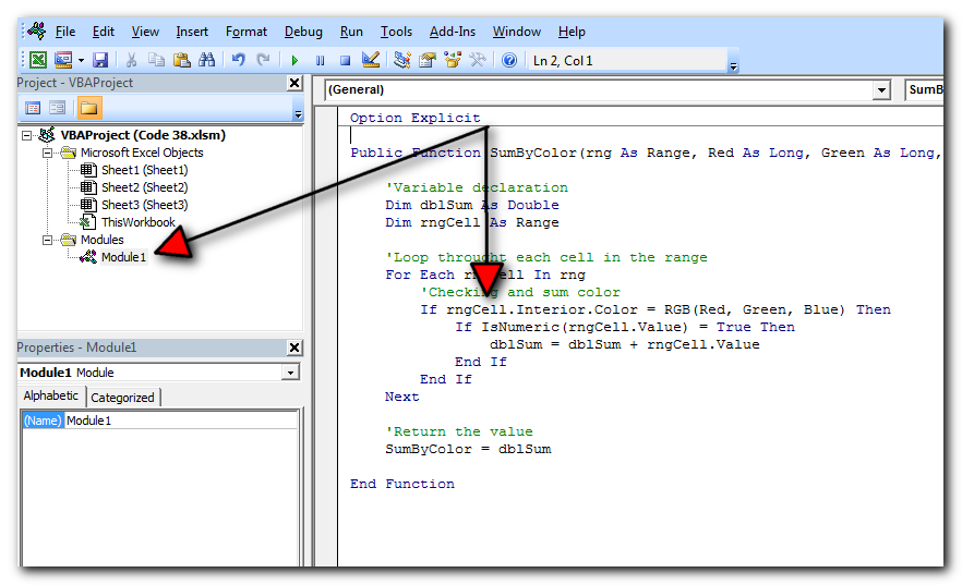
Step 5: Now you are ready to use this code as Excel Function/Formula
Step 6: Type the formula in the cell where you want to get the sum specific colored cells
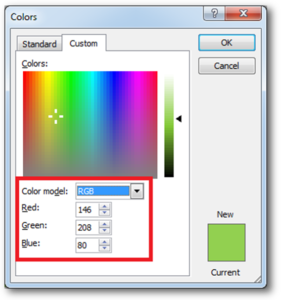
First Code Example: =SumByColor(A2:A11,146, 208, 80)
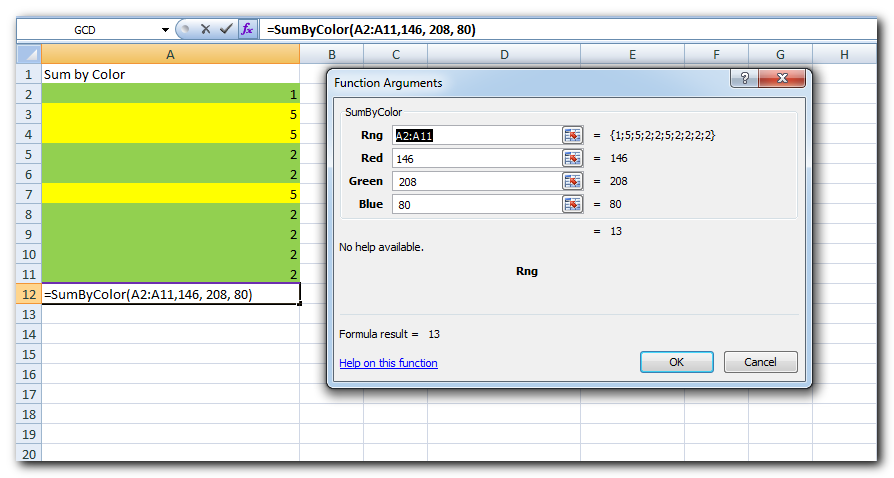
The first parameter of the formula is the range from which you want to sum the specific color cells. The second, third and fourth parameters are RGB code of the color.
Second Code Example: =SumByColor(A2:A11,A3)
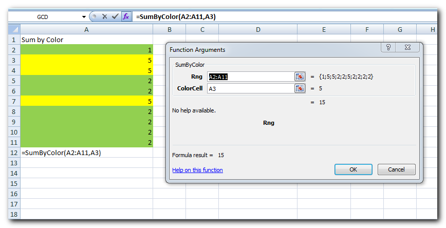
The first parameter of the formula is the range from which you want to sum the specific color cells. The second parameter is the cell from which you want to compare the color.
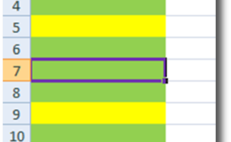
Step 1: Select the cell which contain the color you want to use
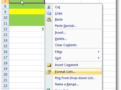
Step 2: Right click and select ‘Format Cells…’
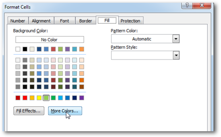
Step 3: In the Format Cells dialog box go to ‘Fill’ tab and click on ‘More Colors…’
Step 4: That’s all, in the ‘Color’ dialog box, you can view the RGB (Red, Green, Blue) codes of the color
Thanks for reading the article, subscribe us to get more VBA tricks

Here we are coming with one more exciting post which can help you to solve very basic but very important problems while writing VBA codes.

Index Match in Excel are powerful tools for advanced lookups. They’re popular because they’re incredibly flexible. You can use them to search horizontally or vertically, perform two-way searches, find values to the left of your search criteria, handle case-sensitive searches, and even search using multiple conditions. If you want to improve your Excel skills, mastering INDEX and MATCH is essential. Below, you’ll find numerous examples to help you grasp how they function.

Free File Renamer Tool – Quickly Rename files batch using Excel VBA Here is another help code and tool for programmers to rename files. You can use this tool for renaming all files available in…

Custom Calendar Control for MS Access MS Access by default provides inbuilt functionality to pick dates using calendar control; however it lacks few basic functionalities which makes selecting a date bit difficult. For example, if…

VBA to Read Excel Data Using Connection String Sometimes as a programmer you need to read heavy (more then 5 MB) Excel files. There are two ways you can read data from Excel files: Open…

VBA Code to send Outlook Emails Sending bulk emails is a very common activity, there are many office activities that need a person to send bulk emails to single or multiple recipients. You also may…
Hi,
How to Count (D71) CONDITIONALLY FORMATTED RED COLOR CELL only (D40:D70)?
Pls guide…
Thanks
If you want to count from single cell then formula will be =SumByColor(D71,256,0,0)