The objective of creating drop-down list is to give an option to a user to select the option from the list.
so that it restricts the user to select unwanted entries input.
we can also use drop-down option for creating interactive dashboards for reporting purpose.
STEP 1 :- As we can see on the top we have a data entry form at the bottom we have a dashboard
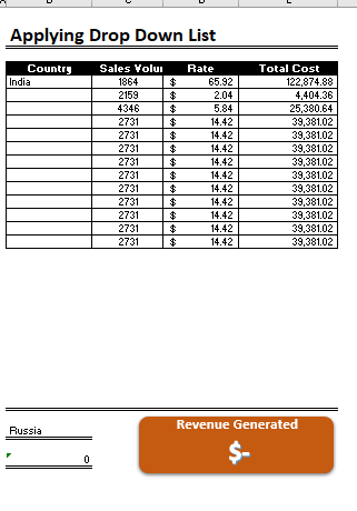
STEP 2 :- So for creating a drop-down list select a cell and go to data under this data there is data validation icon.
now click on the data validation and the screen will pop up shown below.
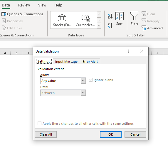
STEP 3 :- Now under the setting option click the allow button and select the list. now in source write the entries for eg india, united states, china etc we can add as many countries than click ok.
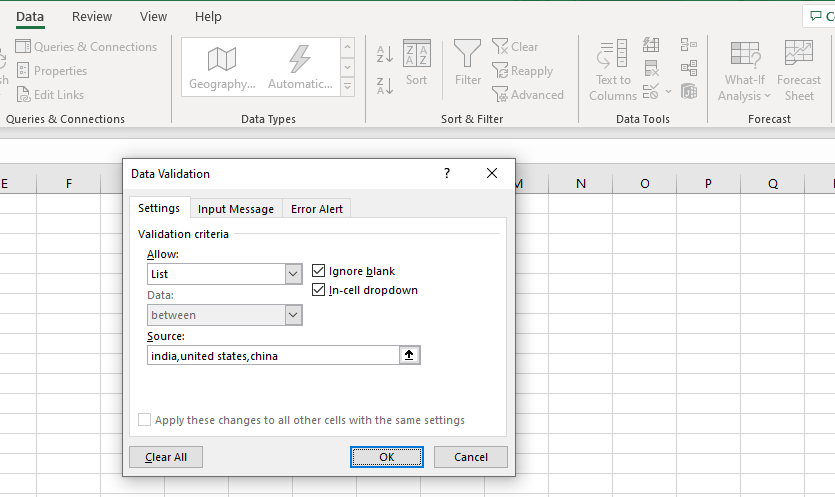
STEP 4 :- Now after this, if we select any cell there is a dropdown list of entries like India,united states, china, etc. so our drop-down list is updated.
Now let us understand how to create a drop-down from the list because whenever we have big data sets than it is not easy to write manually every entry. In this case, We will follow the steps given below.
Step 1: Select the cells containing the headings and values
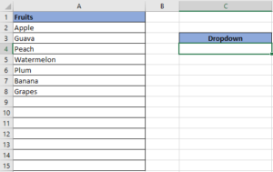
Step 2: Click on “Data” on the top of excel and select Data Validation:

Step 3: Select List under “Allow” and enter the Range of your data under “Source”. Click Ok:
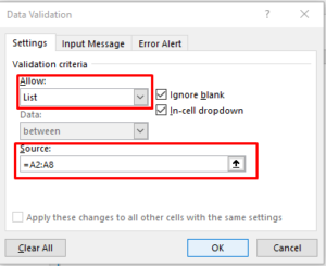
Note: In order to fix the range, you need to use “$” sign before Column and Row reference values i.e. $A$2:$A$8
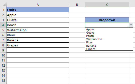
Step 4: Here is your drop down list:

This video will help you to understand how you may use conditional formatting to highlight row based on conditions. Subscribe us for more updates

RANK function performs the Ranking in a range or list of numbers. Function returns the rank position and can assigned as highest or lowest value as 1st Rank

This tutorial will introduce you to a new Excel 365 dynamic array function named CHOOSECOLS and show how you can use it to extract any specific columns from an array. Imagine that you are working…

Print Row Header on Each Page in Excel means that when you print your worksheet, the selected row (often the top row with column headers) will repeat at the top of every printed page. This ensures…
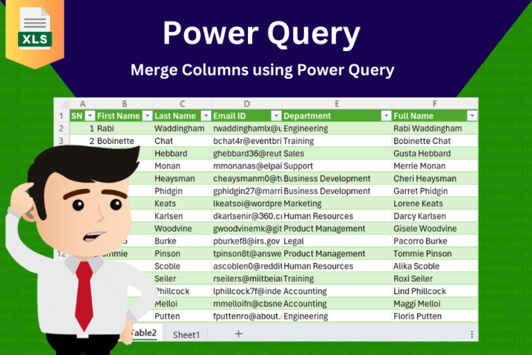
In this tutorial, learn how to merge columns using Power Query. Follow this step-by-step guide to convert data into a table, merge columns seamlessly, and customize separators. Whether you’re a beginner or an advanced user, this tutorial will enhance your data manipulation skills and streamline your workflow. Master Power Query and optimize your data management processes effortlessly.

This tutorial explains how the TRANSPOSE function works and shows you the right way to use it to switch data in Excel.
Everyone has different preferences, even for work habits. Some people like to arrange data in vertical columns, while others prefer horizontal rows. If you ever need to switch the direction of your data quickly, the TRANSPOSE function can help