The objective of creating drop-down list is to give an option to a user to select the option from the list.
so that it restricts the user to select unwanted entries input.
we can also use drop-down option for creating interactive dashboards for reporting purpose.
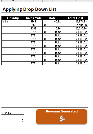
STEP 1 :- As we can see on the top we have a data entry form at the bottom we have a dashboard
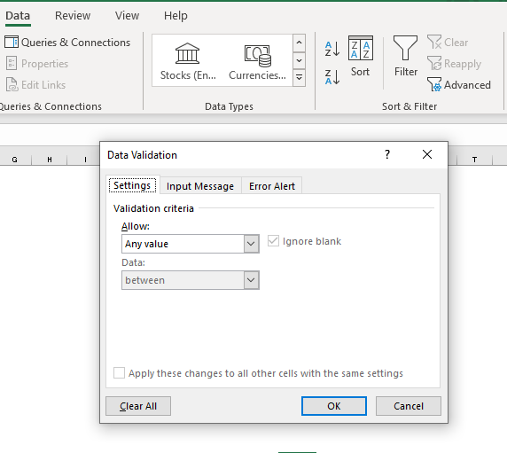
STEP 2 :- So for creating a drop-down list select a cell and go to data under this data there is data validation icon.
now click on the data validation and the screen will pop up shown below.
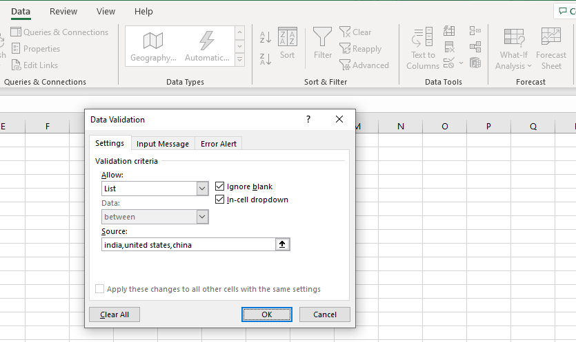
STEP 3 :- Now under the setting option click the allow button and select the list. now in source write the entries for eg india, united states, china etc we can add as many countries than click ok.
STEP 4 :- Now after this, if we select any cell there is a dropdown list of entries like India,united states, china, etc. so our drop-down list is updated.
Now let us understand how to create a drop-down from the list because whenever we have big data sets than it is not easy to write manually every entry. In this case, We will follow the steps given below.
Step 1: Select the cells containing the headings and values
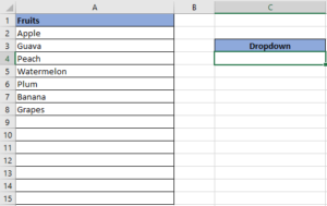
Step 2: Click on “Data” on the top of excel and select Data Validation:

Step 3: Select List under “Allow” and enter the Range of your data under “Source”. Click Ok:
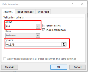
Note: In order to fix the range, you need to use “$” sign before Column and Row reference values i.e. $A$2:$A$8
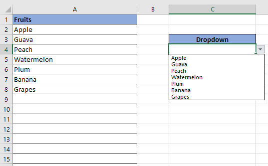
Step 4: Here is your drop down list:
Lock Cells to avoid editing, Hide Formulas Sometimes you create amazing projects, dashboards however people can make mistakes and edit the calculations, formats what you have made. Still you can protect the sheets, workbooks and…

In Excel, a line break lets you finish one line of text and begin another within the same cell. It helps create separate lines of information without needing to move to a different cell.
Use Excel’s DATE function when you need to take three separate values and combine them to form a date.
This tutorial explains what an Excel name is and shows you how to define a name for a cell, range, constant, or formula. You’ll also learn how to edit, filter, and delete defined names in Excel.
Excel names are a bit of a paradox: they’re one of the most useful features, but many people find them unnecessary or too technical. That’s because few users truly understand what Excel names can do. This tutorial will not only teach you how to create a named range in Excel but also show you how this feature can make your formulas easier to write, read, and reuse.

RANK function performs the Ranking in a range or list of numbers. Function returns the rank position and can assigned as highest or lowest value as 1st Rank

Video: How to Hide Worksheet in Excel? Hide Sheet in Excel When I was creating an excel dashboard, there were multiple sheets which I used for calculation purpose and never wanted anybody to make any…