The objective of creating drop-down list is to give an option to a user to select the option from the list.
so that it restricts the user to select unwanted entries input.
we can also use drop-down option for creating interactive dashboards for reporting purpose.
STEP 1 :- As we can see on the top we have a data entry form at the bottom we have a dashboard
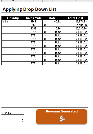
STEP 2 :- So for creating a drop-down list select a cell and go to data under this data there is data validation icon.
now click on the data validation and the screen will pop up shown below.
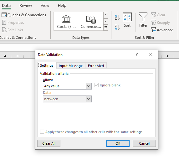
STEP 3 :- Now under the setting option click the allow button and select the list. now in source write the entries for eg india, united states, china etc we can add as many countries than click ok.
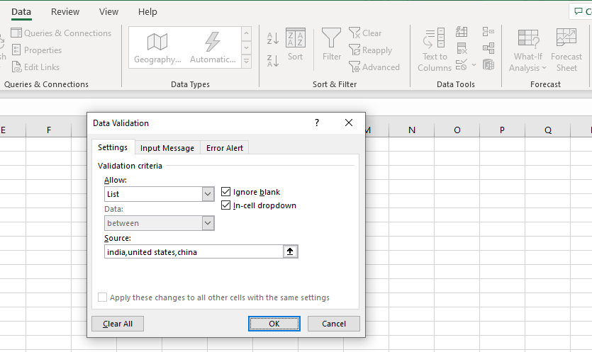
STEP 4 :- Now after this, if we select any cell there is a dropdown list of entries like India,united states, china, etc. so our drop-down list is updated.
Now let us understand how to create a drop-down from the list because whenever we have big data sets than it is not easy to write manually every entry. In this case, We will follow the steps given below.
Step 1: Select the cells containing the headings and values
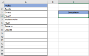
Step 2: Click on “Data” on the top of excel and select Data Validation:

Step 3: Select List under “Allow” and enter the Range of your data under “Source”. Click Ok:
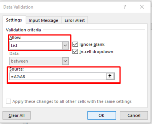
Note: In order to fix the range, you need to use “$” sign before Column and Row reference values i.e. $A$2:$A$8
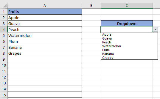
Step 4: Here is your drop down list:
Undo in excel very useful If you’re new to Excel or even if you’ve been using it for a while, you’ve probably made a mistake on a spreadsheet. Mistakes happen a lot, especially when working…

AVERAGEIF function is used to get the “average” of values for matching criteria across range. Average = Sum of all values / number of items.

Excel Function DATE When you work with dates in Excel, the DATE function is crucial to understand. The reason is that some other Excel functions may not always recognize dates when they are entered as…

Introduction Welcome to this comprehensive guide on using Power Query in Excel to split data efficiently. In this tutorial, we’ll walk you through the step-by-step process of splitting columns, specifically focusing on splitting the name…

If you need to keep This quick guide explains what Excel circular references are and why you should be careful when using them. You’ll also learn how to check for, find, and remove circular references in Excel worksheet.a circular reference, it will show you how to turn on and use circular formulas safely
You tried to enter a formula in your Excel sheet, but it’s not working. Instead, Excel is showing you a message about a circular reference. Is that why you’re here? 🙂
Thousands of people run into this issue every day because they accidentally make an Excel formula try to calculate its own cell. When this happens, Excel gives the following error message:

To subtract numbers in Excel, follow these steps:
Start by typing an equal sign (=) in the cell where you want the result.
Enter the first number or cell reference you want to subtract from.
Type a minus sign (-).
Enter the second number or cell reference you want to subtract.