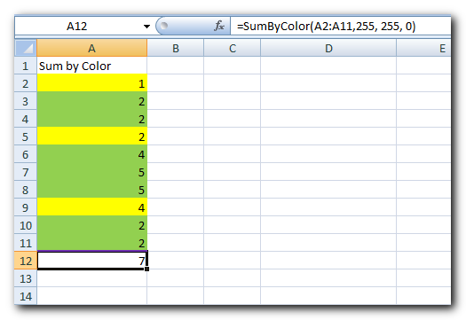
Recently some of our subscribers have requested us to share a VBA code that can sum the cells by its color. To help our subscribers and developers, we are sharing 2 codes that be used to sum the cells with specific color and returns the total sum of the matching color cells
Public Function SumByColor(rng As Range, Red As Long, Green As Long, Blue As Long) As Double

    'Variable declaration
    Dim dblSum As Double
    Dim rngCell As Range

    'Loop throught each cell in the range
    For Each rngCell In rng
        'Checking and sum color
        If rngCell.Interior.Color = RGB(Red, Green, Blue) Then
            If IsNumeric(rngCell.Value) = True Then
                dblSum = dblSum + rngCell.Value
            End If
        End If
    Next

    'Return the value
    SumByColor = dblSum

End FunctionPublic Function SumByColor(rng As Range, ColorCell As Range) As Double
'Variable declaration
Dim dblSum As Double
Dim rngCell As Range
'Loop throught each cell in the range
For Each rngCell In rng
'Checking and sum color
If rngCell.Interior.Color = ColorCell.Interior.Color Then
If IsNumeric(rngCell.Value) = True Then
dblSum = dblSum + rngCell.Value
End If
End If
Next
'Return the value
SumByColor = dblSum
End Function
Step 1: Open the Excel file in which you want to copy this code
Step 2: Press Alt+F11 to open VBA editor
Step 3: Insert a new module from Insert > Module menu
Step 4: Paste the code in the module
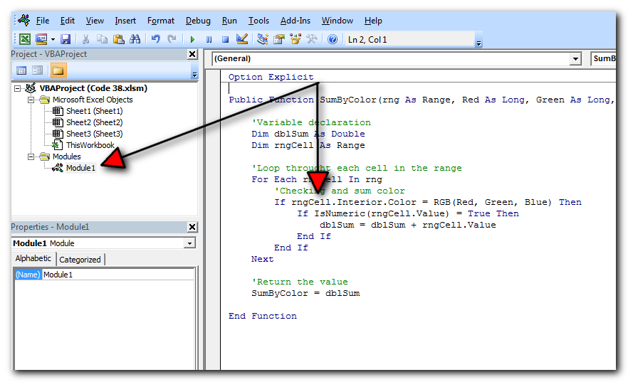
Step 5: Now you are ready to use this code as Excel Function/Formula
Step 6: Type the formula in the cell where you want to get the sum specific colored cells
First Code Example: =SumByColor(A2:A11,146, 208, 80)
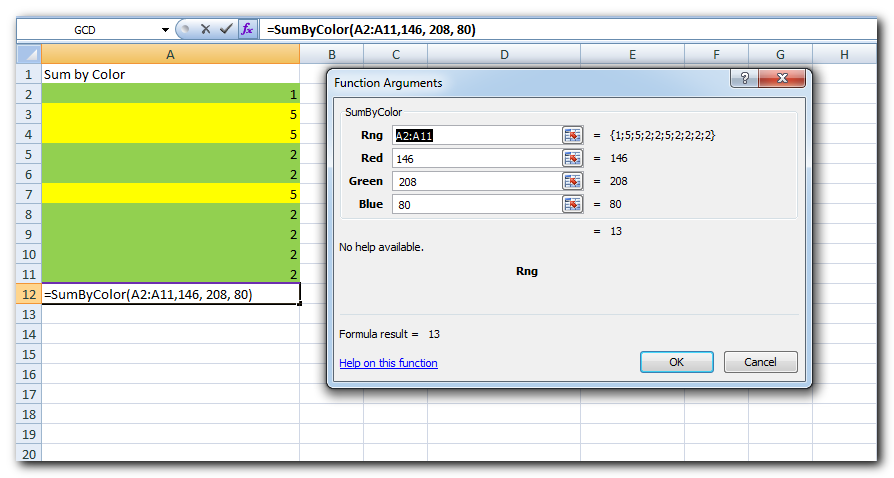
The first parameter of the formula is the range from which you want to sum the specific color cells. The second, third and fourth parameters are RGB code of the color.
Second Code Example: =SumByColor(A2:A11,A3)
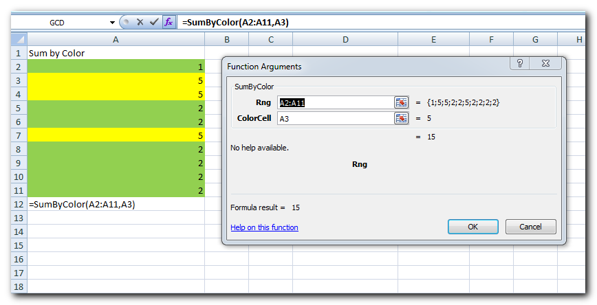
The first parameter of the formula is the range from which you want to sum the specific color cells. The second parameter is the cell from which you want to compare the color.
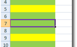
Step 1: Select the cell which contain the color you want to use
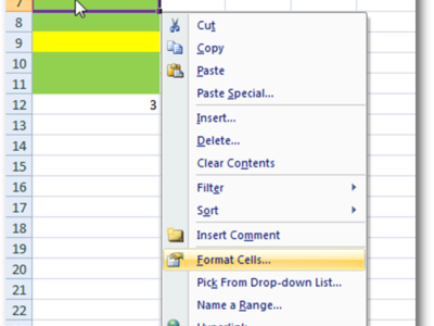
Step 2: Right click and select ‘Format Cells…’
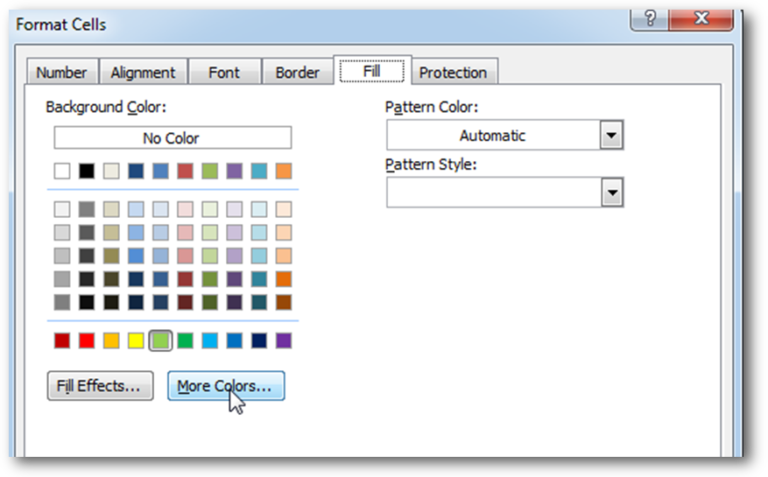
Step 3: In the Format Cells dialog box go to ‘Fill’ tab and click on ‘More Colors…’
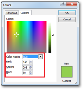
Step 4: That’s all, in the ‘Color’ dialog box, you can view the RGB (Red, Green, Blue) codes of the color
Thanks for reading the article, subscribe us to get more VBA tricks

VBA Code To Delete All Shapes On A Excel sheet Here is a VBA code which deletes all the shapes from an Excel sheet. Code is simple but you have to be bit careful while…

VBA Code to Sort Data HERE IS A ONE LINE CODE FOR DEVELOPER’S REFERENCE WHICH CAN BE USED TO SORT DATA ‘Sort data in ascending order on Column F (Created At) Sheet1.Range(“A1:G” & Sheet1.Cells.SpecialCells(xlCellTypeLastCell).Row).Sort Key1:=Sheet1.Range(“F1”),…
Time Management is very effective way of managing the available time. Current competitive world is making the time management crucial. There are various ways, tools and techniques by which time management can be done easily.

Here is one more wonderful free tool from ExcelSirJi.com which makes your life easy. Time & Motion Tracker helps you to track Start and End time of any type of transaction or activity. The good thing is, it is VBA based tool which helps you to protect from manual manipulation in the data by the user. It is also easy to use, just click on Start (shortcut: Ctrl+Shift+A) or Stop (Ctrl+Shft+S) buttons to record the time

What is the Usage of sheet color in Excel? When we prepare a report or a dashboard it is easy to identify or analyze reports with a change of color sheet tabs. Analysts generally give…
Time and Motion Tracker is an MS Excel based tool which helps you to track Start and End time of any type of transaction or activity. The tool is developed using VBA coding which helps you to protect manual manipulation in the data by the user. It is also easy to use, just click on Start (shortcut: Ctrl+W) or Stop (Ctrl+E) buttons to record the time stamp. This is professional version of our famous Time & Motion Tracker. This version includes features such as Hold Timer, Consolidation, Utilization Analysis, Dashboards etc.
Hi,
How to Count (D71) CONDITIONALLY FORMATTED RED COLOR CELL only (D40:D70)?
Pls guide…
Thanks
If you want to count from single cell then formula will be =SumByColor(D71,256,0,0)