The objective of creating drop-down list is to give an option to a user to select the option from the list.
so that it restricts the user to select unwanted entries input.
we can also use drop-down option for creating interactive dashboards for reporting purpose.
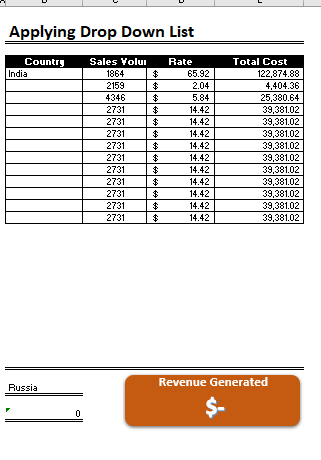
STEP 1 :- As we can see on the top we have a data entry form at the bottom we have a dashboard
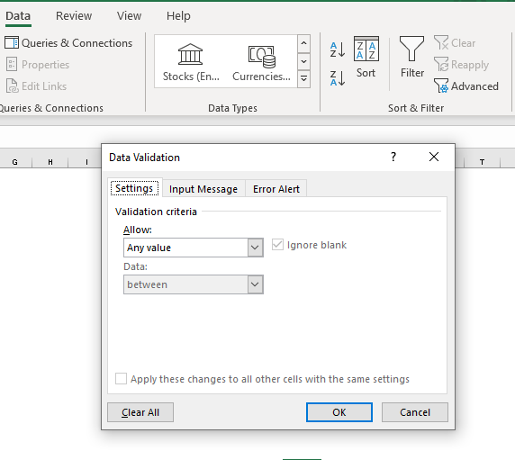
STEP 2 :- So for creating a drop-down list select a cell and go to data under this data there is data validation icon.
now click on the data validation and the screen will pop up shown below.
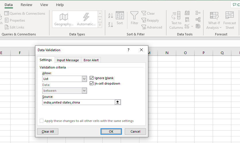
STEP 3 :- Now under the setting option click the allow button and select the list. now in source write the entries for eg india, united states, china etc we can add as many countries than click ok.
STEP 4 :- Now after this, if we select any cell there is a dropdown list of entries like India,united states, china, etc. so our drop-down list is updated.
Now let us understand how to create a drop-down from the list because whenever we have big data sets than it is not easy to write manually every entry. In this case, We will follow the steps given below.
Step 1: Select the cells containing the headings and values
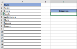
Step 2: Click on “Data” on the top of excel and select Data Validation:

Step 3: Select List under “Allow” and enter the Range of your data under “Source”. Click Ok:
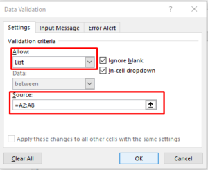
Note: In order to fix the range, you need to use “$” sign before Column and Row reference values i.e. $A$2:$A$8
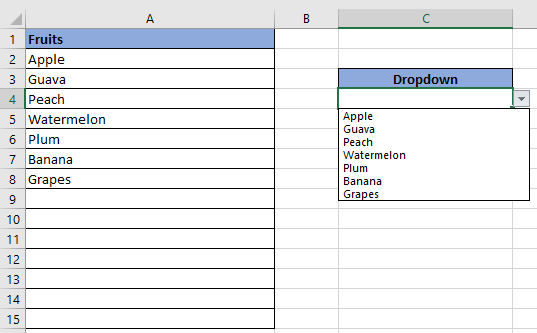
Step 4: Here is your drop down list:
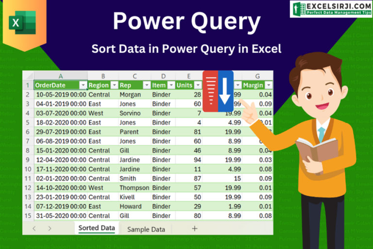
This article unveils the magic of Power Query, a built-in Excel tool that simplifies data organization. Learn how to sort by single or multiple columns, create layered sorts for complex needs, and even reverse your data order entirely. Power Query puts you in control, transforming your data into a well-structured format for effortless analysis.

How to Hide Ribbon &Formula bar in excel? While preparing many projects, my clients always want me to make professional, good looking dashboards. So I hide few things like Gridlines, Column & Row headings and…
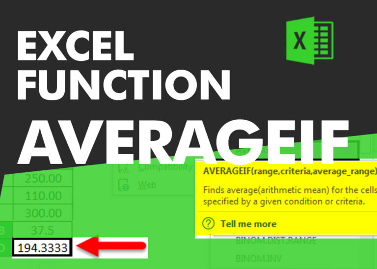
AVERAGEIFS function is used to get the “average” of values for matching criteria across range. Average = Sum of all values / number of items.

This tutorial will introduce you to a new Excel 365 dynamic array function named CHOOSECOLS and show how you can use it to extract any specific columns from an array. Imagine that you are working…

Video: How to Hide Worksheet in Excel? Hide Sheet in Excel When I was creating an excel dashboard, there were multiple sheets which I used for calculation purpose and never wanted anybody to make any…

Scroll Lock in Excel can make scrolling, selecting cells, checking formulas, entering data, and recording macros harder. So, you might need to turn it off to work normally. In this article, we’ll show you how…