The objective of creating drop-down list is to give an option to a user to select the option from the list.
so that it restricts the user to select unwanted entries input.
we can also use drop-down option for creating interactive dashboards for reporting purpose.
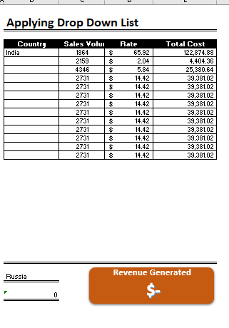
STEP 1 :- As we can see on the top we have a data entry form at the bottom we have a dashboard
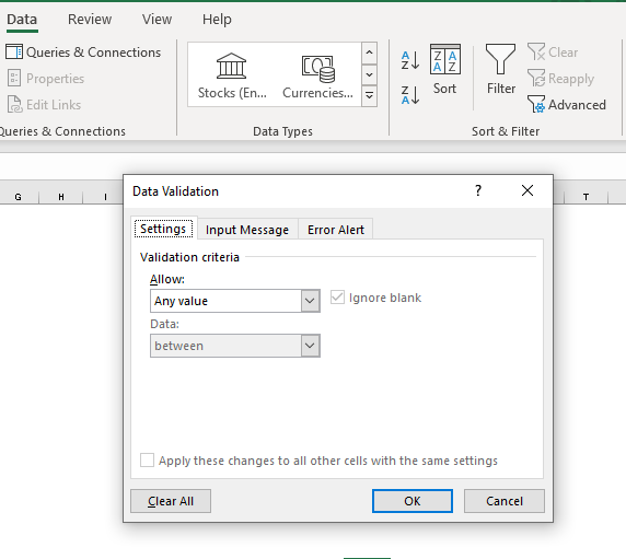
STEP 2 :- So for creating a drop-down list select a cell and go to data under this data there is data validation icon.
now click on the data validation and the screen will pop up shown below.
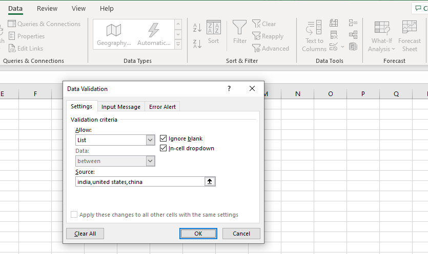
STEP 3 :- Now under the setting option click the allow button and select the list. now in source write the entries for eg india, united states, china etc we can add as many countries than click ok.
STEP 4 :- Now after this, if we select any cell there is a dropdown list of entries like India,united states, china, etc. so our drop-down list is updated.
Now let us understand how to create a drop-down from the list because whenever we have big data sets than it is not easy to write manually every entry. In this case, We will follow the steps given below.
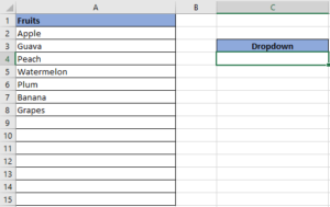
Step 1: Select the cells containing the headings and values
Step 2: Click on “Data” on the top of excel and select Data Validation:

Step 3: Select List under “Allow” and enter the Range of your data under “Source”. Click Ok:
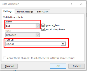
Note: In order to fix the range, you need to use “$” sign before Column and Row reference values i.e. $A$2:$A$8
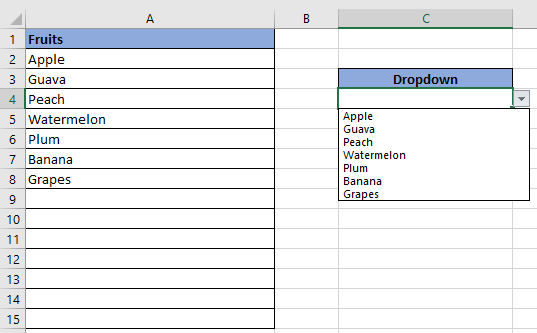
Step 4: Here is your drop down list:

Group worksheets in Excel makes it easier to manage a big workbook. This feature allows you to treat multiple worksheets as one, helping you perform identical tasks like formatting or data entry across several sheets…

AVERAGEIF function is used to get the “average” of values for matching criteria across range. Average = Sum of all values / number of items.

While starting Excelsirji.Com, it is always been critical for me to find the best to amaze the viewer experience. So I spent many hours on web to read, explore amazing excel content which I really…

To subtract numbers in Excel, follow these steps:
Start by typing an equal sign (=) in the cell where you want the result.
Enter the first number or cell reference you want to subtract from.
Type a minus sign (-).
Enter the second number or cell reference you want to subtract.

In an “IF function” there will be two output i.e. TRUE or FALSE since either the statement will be “TRUE” or “FALSE”. If the statement is matching or correct, then output will be “TRUE” or if the statement is not matching or not correct then the output will be “FALSE

Today, I’ll show you how to add bullet points in Excel with simple steps and clear images, so you can easily highlight key points in your Excel reports for better clarity and readability. Bullet points…